XRONOS is a worldwide database of chronological data (such as radiocarbon or dendrochronological dates) from archaeological contexts. The xronos package allows you to retrieve data from XRONOS directly using R. It also provides tools for inspecting and transforming this data for analysis with commonly-used packages.
This vignette introduces the main features of the xronos package. It covers:
- Querying and retrieving chronological data from XRONOS with
chron_data() - Calibrating radiocarbon dates with xronos and c14
- Mapping chronological data with xronos and sf
Get chronological data
chron_data() provides an R interface to XRONOS’ REST API for retrieving
chronological data. Without further parameters, it will request all
available data from XRONOS.
Since this takes some time, you will be prompted to confirm this
request. Use chron_data(.everything = TRUE) to confirm that
you do want to download all records from XRONOS and suppress this
prompt.
In practice, you’ll probably want to narrow down the dataset with a
search query. You can use the following parameters, passed as arguments
to chron_data(), to filter the results:
labnrsitesite_type-
country(ideally a two-letter country code, otherwise the function will attempt to interpret it as one using countrycode::countryname()) featurematerialspecies
You can combine any number of parameters, and each parameter can take either a single value or a vector of values that should be included in the results.
For example, to get all radiocarbon dates from Switzerland on either charcoal or bone:
chron_ch <- chron_data(country = "CH", material = c("charcoal", "bone"))The results of the query are returned as a table of records (a
tibble if tibble is installed, otherwise a data frame):
chron_ch
#> # A tibble: 3,320 × 20
#>       id labnr        bp   std source_database lab_name material species
#>    <dbl> <chr>     <dbl> <dbl> <chr>           <chr>    <chr>    <chr>
#>  1  4946 ETH-63150  9044    35 ""              ""       charcoal Corylus avella…
#>  2  4946 ETH-63150  9044    35 ""              ""       charcoal Corylus avella…
#>  3  4947 ETH-63685  8912    33 ""              ""       charcoal Corylus avella…
#>  4  4947 ETH-63685  8912    33 ""              ""       charcoal Corylus avella…
#>  5  4948 ETH-63687  8909    47 ""              ""       charcoal Ulmus
#>  6  4948 ETH-63687  8909    47 ""              ""       charcoal Ulmus
#>  7  4949 ETH-63686  8812    33 ""              ""       charcoal Prunus
#>  8  4949 ETH-63686  8812    33 ""              ""       charcoal Prunus
#>  9  5070 VERA-2905   235    35 ""              ""       charcoal NA
#> 10  5070 VERA-2905   235    35 ""              ""       charcoal NA
#> # ℹ 3,310 more rows
#> # ℹ 12 more variables: feature_type <chr>, site <chr>, country <chr>,
#> #   site_type <chr>, periods <list>, typochronological_units <list>,
#> #   ecochronological_units <list>, reference <list>, lat <chr>, lng <chr>,
#> #   delta_c13 <dbl>, feature <chr>
Calibrating radiocarbon data
There are several R packages that include functions for radicarbon
calibration, including rcarbon, oxcAAR (requires external software), and
BChron. Calibrating radiocarbon data from XRONOS should follow the same
general principle whichever is used: pass the columns bp
and std—and possibly also labnr as a unique
ID—as arguments to the calibration function. For example, using
rcarbon:
library(rcarbon)

chron_moos <- chron_data(site = "Moos")
chron_moos <- unique(chron_moos[c("labnr", "bp", "std")]) # Remove duplicates

chron_moos_cal <- calibrate(x = chron_moos$bp,
                            errors = chron_moos$std,
                            ids = chron_moos$labnr,
                            verbose = FALSE)
The results are best understood using a plot:
multiplot(chron_moos_cal)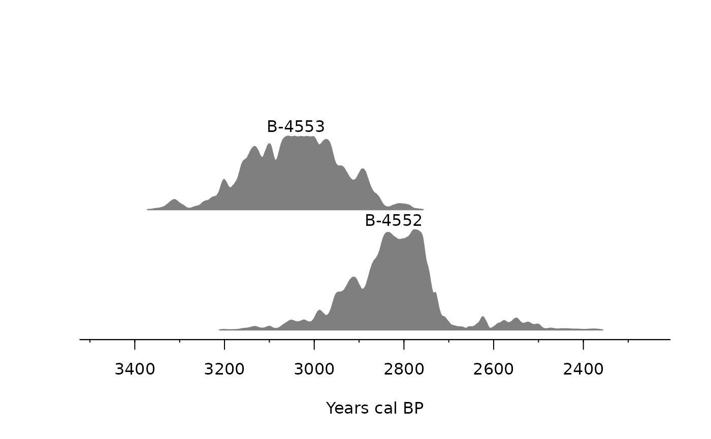
Map chronological data
Wherever possible, XRONOS includes the geographic location of chrons,
stored as latitude and longitude coordinates. The convenience function
chron_as_sf() converts these coordinates into a ‘simple
features’ geometry column for use with the sf package:
library(sf)
#> Linking to GEOS 3.12.1, GDAL 3.8.4, PROJ 9.4.0; sf_use_s2() is TRUE

chron_as_sf(chron_ch)
#> Warning: 1103 rows with missing or invalid coordinates were removed.
#> Simple feature collection with 2217 features and 20 fields
#> Geometry type: POINT
#> Dimension:     XY
#> Bounding box:  xmin: 6.1419 ymin: 45.96543 xmax: 10.38184 ymax: 47.75
#> Geodetic CRS:  WGS 84
#> # A tibble: 2,217 × 21
#>       id labnr        bp   std source_database lab_name material species
#>  * <dbl> <chr>     <dbl> <dbl> <chr>           <chr>    <chr>    <chr>
#>  1  5204 ETH-16449  4370    70 ""              ""       charcoal NA
#>  2  5204 ETH-16449  4370    70 ""              ""       charcoal NA
#>  3  5205 ETH-18123  4365    65 ""              ""       charcoal NA
#>  4  5205 ETH-18123  4365    65 ""              ""       charcoal NA
#>  5  5206 ETH-18124  4720    60 ""              ""       charcoal NA
#>  6  5206 ETH-18124  4720    60 ""              ""       charcoal NA
#>  7  5207 ARC-1100   4490    55 ""              ""       charcoal NA
#>  8  5207 ARC-1100   4490    55 ""              ""       charcoal NA
#>  9  5208 B-4703     4430    40 ""              ""       charcoal NA
#> 10  5208 B-4703     4430    40 ""              ""       charcoal NA
#> # ℹ 2,207 more rows
#> # ℹ 13 more variables: feature_type <chr>, site <chr>, country <chr>,
#> #   site_type <chr>, periods <list>, typochronological_units <list>,
#> #   ecochronological_units <list>, reference <list>, lat <chr>, lng <chr>,
#> #   delta_c13 <dbl>, feature <chr>, geometry <POINT [°]>
The result is an sf object, which includes the original
data, plus a geometry column representing the point coordinates and
information on the coordinate reference system used.
Change the crs parameter to transform the geometries
into another coordinate reference system. This can be anything
understood by sf::st_crs()). For example, to use the Swiss
National Grid (EPSG:2056):
chron_as_sf(chron_ch, crs = 2056)
#> Warning: 1103 rows with missing or invalid coordinates were removed.
#> Simple feature collection with 2217 features and 20 fields
#> Geometry type: POINT
#> Dimension:     XY
#> Bounding box:  xmin: 2499921 ymin: 1090462 xmax: 2825381 ymax: 1289561
#> Projected CRS: CH1903+ / LV95
#> # A tibble: 2,217 × 21
#>       id labnr        bp   std source_database lab_name material species
#>  * <dbl> <chr>     <dbl> <dbl> <chr>           <chr>    <chr>    <chr>
#>  1  5204 ETH-16449  4370    70 ""              ""       charcoal NA
#>  2  5204 ETH-16449  4370    70 ""              ""       charcoal NA
#>  3  5205 ETH-18123  4365    65 ""              ""       charcoal NA
#>  4  5205 ETH-18123  4365    65 ""              ""       charcoal NA
#>  5  5206 ETH-18124  4720    60 ""              ""       charcoal NA
#>  6  5206 ETH-18124  4720    60 ""              ""       charcoal NA
#>  7  5207 ARC-1100   4490    55 ""              ""       charcoal NA
#>  8  5207 ARC-1100   4490    55 ""              ""       charcoal NA
#>  9  5208 B-4703     4430    40 ""              ""       charcoal NA
#> 10  5208 B-4703     4430    40 ""              ""       charcoal NA
#> # ℹ 2,207 more rows
#> # ℹ 13 more variables: feature_type <chr>, site <chr>, country <chr>,
#> #   site_type <chr>, periods <list>, typochronological_units <list>,
#> #   ecochronological_units <list>, reference <list>, lat <chr>, lng <chr>,
#> #   delta_c13 <dbl>, feature <chr>, geometry <POINT [m]>
Sometimes you might see a warning about rows with missing or invalid
coordinates being dropped. This is because it is currently not possible
to include rows without a geometry in a simple features table. To
suppress the warning—and clarify your intent—you may want to explicitly
remove these before calling chron_as_sf():
chron_ch |>
  chron_drop_na_coords() |>
  chron_as_sf(crs = 2056) ->
  chron_ch
sf and related packages offer many options for manipulating,
analysing, and mapping spatial data. As a simple example, we can plot
the location of our dates using their natural projection (here we use
sf::st_geometry() to plot only the points themselves, not
their data attributes):
plot(sf::st_geometry(chron_ch), graticule = TRUE, axes = TRUE)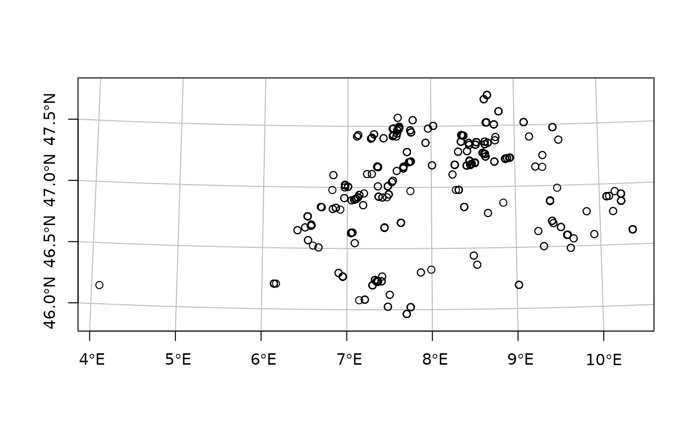
See the sf documentation for more options for plotting simple features.
sf objects generally act like data frames, but if
necessary you can explicitly restore the plain table of data with
sf::st_drop_geometry():
chron_ch <- st_drop_geometry(chron_ch)Note that this does not restore any records that were
dropped by chron_as_sf().